Of course, this is a followup to my previous post, but it merits a separate entry, I think.

It was only natural that I would want to push ahead to 6 from 5, but to do so, I abandoned my application of the “pivot principle” for a more simple and predictable “aufbau” technique, in which we add the 12 component 5-cubes one by one to build up all possible connected subsets of 2, 3, 4, …, 12 of which the last represents the possible unfoldings.

The simple principle is that all cubes are equivalent among the remaining pairs where neither member has been added. This limits the combinatorial excess of multiple versions of equivalent configurations under the symmetry operations of the 6-cube. These operations are the 6! reorderings of the axis labels times the 2⁶  “flips” of the axis orientations, amounting to an impressive 46080 operations.

This number is what creates the time bound for the complete calculation. It took only 4 seconds to generate  2499470 candidate configurations of 12 cubes from the unique canonical representations of the 11 cube configurations:

$ time build1 < cube11 | wc -l
2499470

real 0m4.174s
user 0m4.085s
sys 0m0.124s

… however it took over 8 hours to reduce each of these to its canonical value, requiring just another minute for the final step:

$ time sort -u cube12.canon | wc -l
502110

real 0m28.491s
user 1m37.750s
sys 0m0.310s

…  Of course, I saved the result in a file named cube12 , which has the “grep format” explained in my previous post:

$ head cube12
….00 ….01 ….10 …0.0 …1.0 ..0..0 ..1..0 .0…0 .1…0 0….0 1….0
….00 ….01 ….10 …0.0 …1.0 ..0..0 ..1..0 .0…0 .1…0 0….0 1….1
….00 ….01 ….10 …0.0 …1.0 ..0..0 ..1..0 .0…0 .1…0 0….0 1…0.
….00 ….01 ….10 …0.0 …1.0 ..0..0 ..1..0 .0…0 .1…0 0….0 1…1.
….00 ….01 ….10 …0.0 …1.0 ..0..0 ..1..0 .0…0 .1…0 0….0 1..0..
….00 ….01 ….10 …0.0 …1.0 ..0..0 ..1..0 .0…0 .1…0 0….1 1….1
….00 ….01 ….10 …0.0 …1.0 ..0..0 ..1..0 .0…0 .1…0 0….1 1…0.
….00 ….01 ….10 …0.0 …1.0 ..0..0 ..1..0 .0…0 .1…0 0….1 1…1.
….00 ….01 ….10 …0.0 …1.0 ..0..0 ..1..0 .0…0 .1…0 0….1 1..0..
….00 ….01 ….10 …0.0 …1.0 ..0..0 ..1..0 .0…0 .1…0 0…0. 1…0.

$ tail cube12
….00 …0.0 …11. ..0..1 ..0.1. .0…1 .1.1.. .11… 0..0.. 00…. 1.1…
….00 …0.0 …11. ..0..1 ..0.1. .0…1 .1.1.. 0…0. 0.1… 1..0.. 10….
….00 …0.0 …11. ..0..1 ..0.1. .0…1 .1.1.. 0…0. 00…. 1..0.. 1.1…
….00 …0.0 …11. ..0..1 ..0.1. .0…1 .1.1.. 0…0. 01…. 1..0.. 1.1…
….00 …0.0 …11. ..0..1 ..0.1. .0..0. .1.0.. .11… 0..1.. 0.1… 10….
….00 …0.0 …11. ..0..1 ..0.1. .0..0. .1.0.. .11… 0..1.. 00…. 1.1…
….00 …0.0 …11. ..0..1 ..1.1. .0…1 .1..1. 0…0. 1..0.. 1.0… 11….
….00 …0.0 …11. ..0..1 ..1.1. .0…1 .1.1.. 0…0. 00…. 1..0.. 1.1…
….00 …0.0 …11. ..0..1 ..1.1. .0..0. .1.0.. .10… 0..1.. 00…. 1.1…
….00 …0.0 …11. ..0..1 ..1.1. .0..0. .1.0.. .10… 0..1.. 1.1… 10….

VISUALIZING THE 6-CUBE

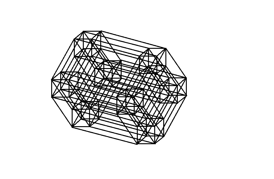
OK, there are 502110 canonically unique unfoldings of the 6-cube into 5-cubes, but what does this even mean? Can we picture it in any way? I think we can! Although 6 orthogonal axes are a challenge to ones powers of visualization. Here was a first attempt at it:

I should note that this is an example of Oblique Projection, which allows great latitude. Essentially, one can pick a “star” of any six line segments as representations of the six orthogonal unit vectors, with the only requirement being that each edge is represented by a parallel displacement of one of these.

Well, we can see that there are four tesseracts there, connected in a ring, but it really has the appearance of a “rat’s nest” and it does not make an attractive working model.

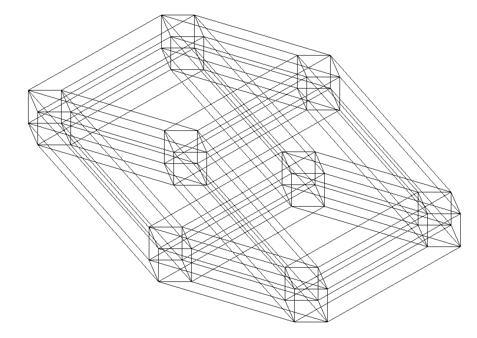
Much better is the idea I had of a “cubed cube” – a large cube whose corners are each split into a small cube whose vertices inherit the connections of the large cube. This is really just a refinement of the above, but a big improvement:

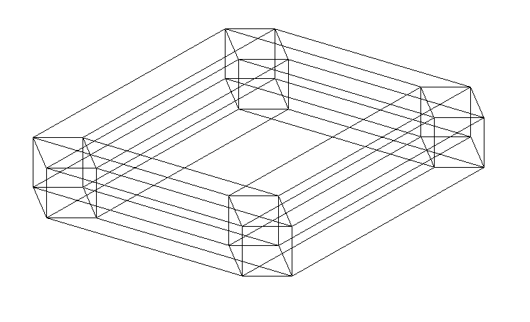
Now we come to the step of finding 5-cubes to use as building blocks for the unfoldings, and it just falls into our lap! There are six each of two varieties of 5-cubes evident. We will choose one of the six “cubed” faces of the large cube:

It is a “cubed square”. Can you see the other six 5-cubes? They each consist of 8 corresponding faces of the small cubes, connected by four large cubes, one at each corner. We needn’t worry about them, though, because all we need is the one we have, and all connections of the unfolding are made by parallel displacements along the 5 axes.

The two axes forming the large square provide a representation of the planar unfoldings of the 3-cube, with the connections formed by the overlap of the “edges” ( which are tesseracts. ) The other three axes are the axes of of the small cubes, which stack ( four at a time ) face to face to form a representation of the cubic unfolding of the tesseract.

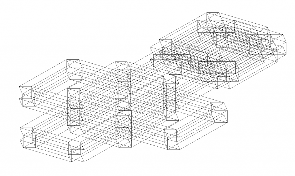
Taken together, these comprise 5 independent lines of connection, but the split into a 2-d plus a 3-d component makes the job feasible as a manual step-by-step process using MS paint. Here is one result, arbitrarily produced:

This is 178th in the sorted list of 502210 canonical unfoldings. It’s early appearance can be accounted for by the simplicity of the scheme used, which relies exclusively on direct opposition of pairs.

178: ….00 ….01 ….10 …0.0 …1.0 ..0..0 ..1..0 .0…1 .1…1 0….1 1….1